One-sentence Summary

Representing four research groups, the authors provide an overview of the shift in acoustic modeling for speech recognition, where deep feedforward neural networks with many hidden layers trained using novel methods replace Gaussian mixture models to estimate HMM state posterior probabilities, yielding significant improvements on a variety of benchmarks.

Key Contributions

• The paper summarizes results from four research groups, showing that deep neural network acoustic models consistently outperform Gaussian mixture models on TIMIT and five large-vocabulary continuous speech recognition tasks, sometimes by large margins.
• Unsupervised pre-training methods (stacked restricted Boltzmann machines or regularized autoencoders) are described; pre-training reduces overfitting and accelerates discriminative fine-tuning, but careful random weight initialization can achieve similar training time reductions.
• The main performance gains are attributed to the deep networks' ability to exploit information across neighboring frames and to model tied context-dependent states, with pre-training acting primarily as a regularizer.

Introduction

The authors focus on acoustic modeling for automatic speech recognition, where Gaussian mixture models paired with hidden Markov models (GMM‑HMMs) have long been the standard. GMMs are statistically inefficient at capturing data that lie on or near a nonlinear manifold, a property common in speech, which limits further accuracy gains. The authors review a two‑stage training procedure that uses deep neural networks (DNNs) to overcome this weakness: unsupervised generative pre‑training of layers is followed by discriminative fine‑tuning to predict HMM states. Applied across multiple research groups, the DNN‑based approach significantly outperforms highly tuned GMM‑HMM systems on both small‑scale and large‑vocabulary continuous speech recognition tasks.

Method

The authors describe a comprehensive method for training Deep Neural Networks (DNNs) that addresses the optimization challenges inherent in deep architectures, such as vanishing gradients and overfitting. While DNNs can be trained discriminatively using backpropagation and stochastic gradient descent (SGD) with momentum, deep networks often struggle to find good weight configurations from random initialization. To overcome this, the authors propose a pipeline consisting of generative pre-training followed by discriminative fine-tuning.

Generative Pre-training with Restricted Boltzmann Machines

The pre-training phase involves learning one layer of feature detectors at a time to model the structure of the input data. The authors utilize Restricted Boltzmann Machines (RBMs), which are undirected graphical models with a bipartite structure consisting of visible and hidden units. The joint probability is defined by an energy function $E(\mathbf{v}, \mathbf{h})$E(v,h). For binary data, the energy is defined as: $E(\mathbf{v}, \mathbf{h}) = - \sum_{i \in \text{visible}} a_i v_i - \sum_{j \in \text{hidden}} b_j h_j - \sum_{i, j} v_i h_j w_{ij}$E(v,h)=−∑i∈visible​ai​vi​−∑j∈hidden​bj​hj​−∑i,j​vi​hj​wij​ To learn the weights efficiently, the authors employ Contrastive Divergence (CD), specifically $\text{CD}_1$CD1​. This algorithm approximates the gradient of the log-likelihood by performing a single step of alternating Gibbs sampling. It starts with a training vector, computes hidden states, reconstructs the visible states, and updates weights based on the difference between data and reconstruction correlations: $\Delta w_{ij} = \epsilon (<v_i h_j>_{\text{data}} - <v_i h_j>_{\text{recon}})$Δwij​=ϵ(<vi​hj​>data​−<vi​hj​>recon​)

For real-valued acoustic data like MFCCs, the authors use a Gaussian-Bernoulli RBM (GRBM). The energy function is modified to include Gaussian noise for visible units: $E(\mathbf{v}, \mathbf{h}) = \sum_{i \in \text{vis}} \frac{(v_i - a_i)^2}{2 \sigma_i^2} - \sum_{j \in \text{hid}} b_j h_j - \sum_{i, j} \frac{v_i}{\sigma_i} h_j w_{ij}$E(v,h)=∑i∈vis​2σi2​(vi​−ai​)2​−∑j∈hid​bj​hj​−∑i,j​σi​vi​​hj​wij​ During training, data is normalized to zero mean and unit variance, and $\sigma_i$σi​ is set to 1 to avoid the complexity of learning noise levels.

Stacking RBMs to Form a Deep Belief Network

To build a deep architecture, the authors stack multiple RBMs. The hidden states of a trained RBM serve as the visible data for training the next RBM. This layer-wise process captures progressively complex statistical structures. The stack of RBMs is then combined into a single generative model called a Deep Belief Network (DBN). In a DBN, the top two layers form an undirected RBM, while lower layers have directed, top-down connections.

Refer to the framework diagram:

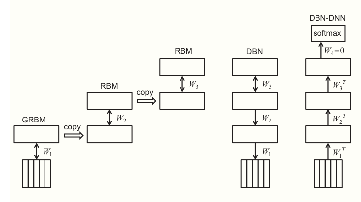
As illustrated in the figure, the process begins with training a GRBM on acoustic coefficients. The hidden states are then used to train subsequent RBMs. Once the stack is complete, the weights are converted to initialize a feed-forward DNN. The undirected connections of lower RBMs are replaced by directed connections (using transposed weights), and a softmax output layer is added.

Discriminative Fine-tuning and HMM Interface

After pre-training, the network is treated as a standard DNN and fine-tuned discriminatively using backpropagation to minimize cross-entropy between predicted and target HMM state probabilities. To interface with an HMM for decoding, the posterior probabilities $P(\text{HMM state} | \text{Acoustic Input})$P(HMM state∣Acoustic Input) output by the DNN are converted to likelihoods $P(\text{Acoustic Input} | \text{HMM state})$P(Acoustic Input∣HMM state) by dividing by the prior state frequencies derived from forced alignment.

The authors also discuss fine-tuning using sequence classification criteria, specifically Maximum Mutual Information (MMI). This optimizes the conditional probability of the entire label sequence given the input sequence, effectively treating the top hidden layer of the DNN as features for a Conditional Random Field. The objective function is: $p(l_{1:T} | v_{1:T}) = \frac{\exp(\sum_{t=1}^T \gamma_{ij} \phi_{ij}(l_{t-1}, l_t) + \sum_{t=1}^T \sum_{d=1}^D \lambda_{l_t, d} h_{td})}{Z(h_{1:T})}$p(l1:T​∣v1:T​)=Z(h1:T​)exp(∑t=1T​γij​ϕij​(lt−1​,lt​)+∑t=1T​∑d=1D​λlt​,d​htd​)​ Gradients are computed with respect to activation parameters, transition parameters, and DNN weights to jointly optimize the system.

Alternative Pre-training Methods

While RBMs are the primary method described, the authors note that other architectures can be used for layer-wise pre-training. Discriminative pre-training, where layers are added and trained sequentially to minimize classification error, is also effective. Additionally, autoencoders can replace RBMs. An autoencoder minimizes the reconstruction error between input and output units, often with a bottleneck code layer.

As shown in the figure below:

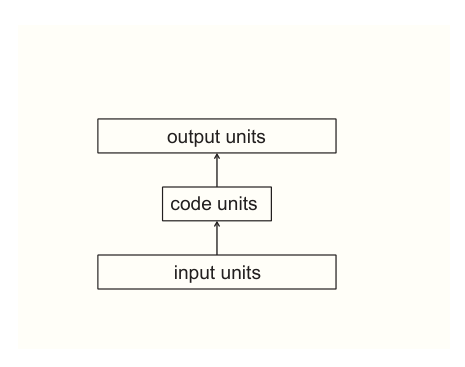
The figure depicts an autoencoder structure with input, code, and output units. Variants like denoising autoencoders (corrupting inputs) or contractive autoencoders (penalizing gradients) are used to regularize the learning process, achieving performance comparable to RBMs in vision tasks, while sparse autoencoders have shown improvements in speech recognition.

Experiment

Deep neural networks with multiple hidden layers, particularly when pre-trained as deep belief networks, consistently outperform Gaussian mixture models across a range of speech recognition tasks, from small-scale phonetic classification on TIMIT to large-vocabulary systems like Bing Voice Search, Switchboard, and broadcast news. These experiments validate that using context-dependent tied triphone states as targets, leveraging multiple frames of acoustic input, and employing deeper architectures all contribute to substantial error reductions. Further investigations show that DNNs can also serve as effective feature extractors for GMM-HMM systems or as detectors of articulatory features, and that convolutional DNNs offer robustness to speaker and noise variability. Overall, the findings confirm that DNN-based acoustic models provide significant and consistent gains over state-of-the-art discriminatively trained GMM-HMM baselines.

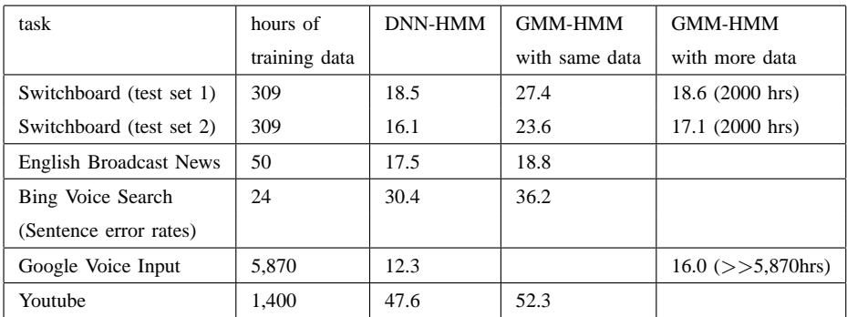
Across five large vocabulary tasks, DNN-HMM systems consistently produced lower word error rates than GMM-HMMs trained on the same amount of data. When GMM-HMMs were given much more training data they could approach DNN-HMM performance, but DNN-HMMs still held an advantage on most tasks. The DNN-HMM achieved a 17.5% word error rate on English Broadcast News with only 50 hours of training, which was the best reported result for that setup. DNN-HMMs yielded lower error rates than GMM-HMMs trained on the same data across all five tasks, with relative improvements ranging from about 7% to over 30%. On the English Broadcast News task with only 50 hours of training data, the DNN-HMM achieved a 17.5% word error rate, which the paper reports as the best result on that benchmark.

Using AE-BN features consistently improved word error rates over GMM-HMM baselines across all LVCSR stages and both 50-hour and 430-hour training conditions. The absolute gain was more pronounced on the smaller dataset, and model combination of the two systems yielded additional reductions, confirming their complementary information. AE-BN features provided larger relative WER improvements on 50 hours of data than on 430 hours after full adaptation. Combining AE-BN and baseline systems further reduced WER, demonstrating complementarity between the approaches.

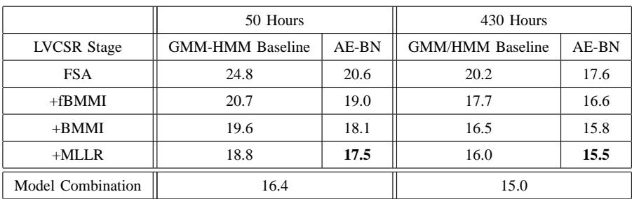
In large vocabulary speech recognition experiments, DNN-HMM and systems using autoencoder bottleneck features were compared against GMM-HMM baselines. Both approaches consistently yielded lower word error rates, with the relative improvements being larger on smaller training sets; the DNN-HMM set a new state-of-the-art on a 50-hour English Broadcast News task, and the autoencoder features showed complementary value when combined with baseline models.